

On 25 August 2026, Oklahoma elected its next governor, or we might safely presume that it has. After the primaries in June showed a Republican electorate split among five major candidates, the election moved to a second round, a one-on-one face-off between the two leading candidates, Gentner Drummond and Mike Mazzei.
While Gentner Drummond was favored in the long campaign season leading into the first round, bettors on Polymarket put his odds of winning the primary at somewhere between 10 and 30% at various points during the 2nd round. Call it the Trump effect. While Polymarket probably overrated Mazzei’s odds based on an overly broad reading of the national environment—he only ended up winning by 2,047 votes—Mazzei did nonetheless prevail against Drummond, pulling off a victory that would have seemed implausible but for Trumpus ex machina.1
Mazzei will now have the privilege of facing off against the Democrats’ latest long shot in the general election. This year, that candidate is House Minority Leader Cyndi Munson. Mazzei isn't bad enough to lose a state this Republican, and Munson isn't good enough to make Republicans remember her name in four years.
Congratulations, Governor Mazzei.
However, the results are less interesting than the map. This was the closest election featuring a winning gubernatorial candidate to occur in Oklahoma since 1950, when Democratic nepo baby Johnston Murray won his primary by just 960 votes. Being so close, the 2026 run-off election saw the re-emergence of an electoral pattern so fundamental to Oklahoma that it dates back to the founding of this state.
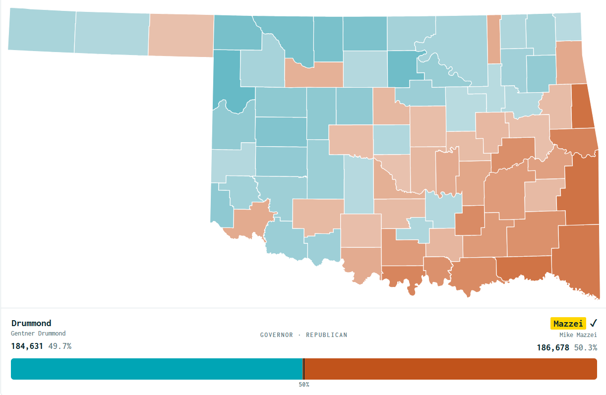
And now, a magic trick! Watch, as one map becomes three! Behold!
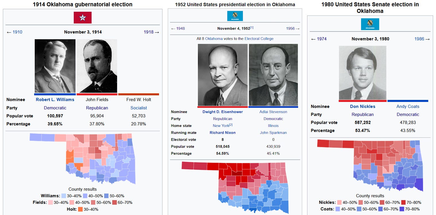
Do you notice something about these maps? One is a gubernatorial election map from 1914, one is a presidential election map from 1952, and one is a Senate election map from 1980. Why put them next to each other? They’re (nearly) the same map: they depict Oklahoma divided along a diagonal line that cuts from Beckham County to Ottawa, tracing the southern peripheries of Tulsa and OKC’s suburbs.
What we are looking at here is a relic: this is what a close general election in Oklahoma has looked like for the entirety of the state’s history.
To demonstrate this point, I pulled the county-by-county election results of every close general election for Presidential electors, Governor, or Senator that has occurred in the history of Oklahoma, “close” being defined as the second place candidate coming within ten points of winning. The first such election was the 1908 presidential election, where the Democratic populist William Jennings Bryan defeated Republican William Taft in Oklahoma, and the most recent was in 2002, when Brad Henry narrowly managed to defeat Steve Largent to become Oklahoma’s most recent Democratic governor.
When you take the average of all these elections and sort counties based on which way they swung, you get a map that looks something like this:
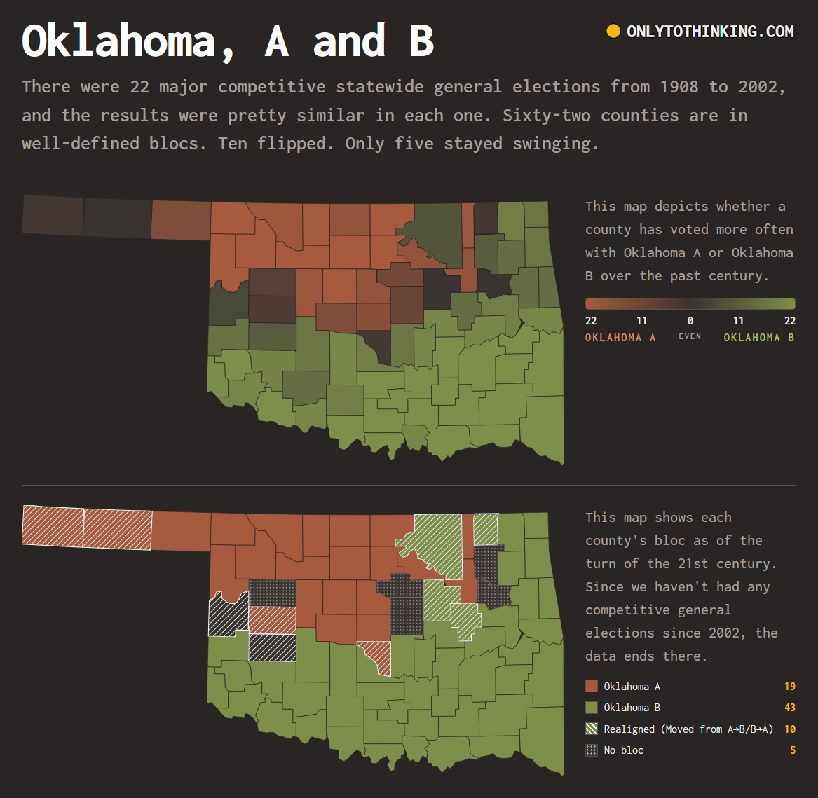
I call this split Oklahoma A and Oklahoma B. OKC, Tulsa, and the northern plains are all in ‘A’, while Little Dixie, Texoma, and the Ozarks are all in ‘B’. From 1908 to 2002, only ten counties jumped from one bloc to the other.
But what is Oklahoma A and B other than an election pattern?
Oklahoma A and B, A Silhouette
Oklahoma A is incorporated. Oklahoma A is wheat fields, shortgrass prairies, section-line roads, and towns where the grain elevators are the tallest thing for forty miles. It’s the descendants of Kansans, Nebraskans, Germans, Mennonites, and Czechs who settled down after the 1893 land run and never left. It’s Enid, Alva, Woodward, Guymon, Ponca City, Bartlesville, and Stillwater. It’s co-ops, refineries, the county fair, and OSU.
Politically, it’s always been conservative, so it’s always been Republican. It voted for Dewey over Roosevelt in ‘44 and then voted for Goldwater over Johnson in ‘64, not by Mississippi margins, but by Arizona margins. ‘A’ politics are the politics of the Chamber of Commerce. It is the politics of the man who owns the elevator, and today, the man who owns the most elevators. It is an old dog that learns new tricks. It’s the boring fiscal conservatism that keeps taxes low, rule books short, and liberals around. It was locked out of power in Oklahoma for most of its history, but it never changed its mind. It built Oklahoma City and Tulsa. It waited until Oklahoma B came around.
Oklahoma B is personal. It’s towns nestled in the foothills of old Indian Territory. It’s timber and rivers and lakes, the Milky Way spilled across night skies above Bigfoot forests. It was the Five Tribes. Now it’s a million tribes, a million families of half-Cherokee, half-Anglo, half-Hillbilly, half-Comanche descent. It’s Durant, Idabel, Antlers, Hugo, Poteau, Ada, Altus, and Hobart. Tribal government, the Baptist church, and the old courthouse with the judge who knows each man who takes the stand.
B was a blue dog, but now, it’s a red dog, or a dog that wears a MAGA hat, or a dog that votes Markwayne Mullin for senator so he can put Teamsters in their place. Back in the midcentury, it was bluer than Massachusetts. Nowadays, it’s redder than Kentucky. A B town’s politics was the politics of the guy who had a beer with the sheriff. These days it’s the politics of the guy who comes straight through the algorithm to make a handheld appeal. It was Gene Stipe, David Boren, and Dan Boren. Now it’s J.J. Humphrey and Donald Trump.
If this is all getting a bit too mushy and poetic for you, I don’t disagree. That’s why I have data.
The Data
When I first noticed this electoral trend that has seen Oklahoma divided the same way so many times, I ran a variety of checks for rigor. In other words, I wanted to make sure that what I was seeing was real.
First, I calculated what’s called a silhouette score, which is a test for how many groups a dataset really has. I ran the test on the county sample to see whether Oklahoma might actually have more than two regions. The results were decisive: no other number of regions scored higher than two, which scored 0.689. Remember that number: the A-B split has a silhouette score of 0.689. Every additional region really just shaved small chunks of three or four counties off of the two main regions—so the number of regions is right.
Next, I tested the split against chance with what’s called a permutation test. I scrambled the county voting records to destroy any pattern in them, then ran a sorting procedure on the scrambled data to see what it could find in pure noise. I did this a thousand times. The luckiest run had a 0.201 silhouette score. Chance never got a third of the way there. Put another way, the split isn’t noise.
Okay, but maybe another method could produce a better, more convincing, or different split. Curious, I checked. In my first draft, I wrote out exactly how each of these methods work, and the essay became unreadable. So I will summarize by saying that I ran six different tests designed to sort data into groups (average linkage, complete linkage, Ward’s method, K-means, spectral clustering, and principal-component sign split), and each of them yielded an extremely similar split, only disagreeing with each other over nine oddball border counties. Map wins again.
The split’s most important victory, however, is its applicability to the 2026 election. Using a set of just 22 elections, the last of which occurred over twenty years ago, I could have predicted how 52/77 counties would have voted in the primary runoff election. I would have had a one in twelve hundred chance of getting that close by random chance. It also correctly predicted every county that selected their candidate by more than twenty points, and 14 of the “misses” were within five points. Not bad!
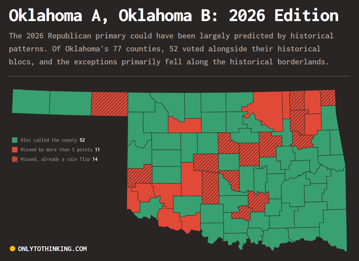
As for the regions that broke with the broad historical pattern in this last election, they tended to break in a historical way: the rural northeast broke for Drummond: they were always the weakest links in the B bloc. The suburban counties—like Comanche, Cleveland, Canadian, Logan, and Washington—favored Mazzei. This makes sense: these counties have changed a lot in the past twenty years of urbanization, so their voting patterns might be expected to change concurrently.
The only real shock came from the southwest. Six counties—Harmon, Greer, Tillman, Cotton, Kiowa, Caddo—sat in B for twenty straight cycles, about as loyal as counties get, and then left together, by an average of twelve points. That’s a story for another time.
Why It Matters — and Why It Might Not
The Oklahoma A-B split matters for a few important reasons.
First, it’s cool to know more stuff, and it’s especially cool to be able to sort stuff into categories. In an era where the D-R partisan split has all but ceased to matter in Oklahoma politics, Oklahoma A-B is a convenient, relatively well-defined, non-partisan categorization that can serve as a catch-all for referring to this very clear political pattern. In the future, I would be interested in researching the origins and effects of the A-B split. Do legislators vote differently or propose different types of legislation based on whether they’re “A” or “B” legislators? Do “A” or “B” county governments operate in a different manner? What’s the origin of the A-B split—is it old settlement patterns, geography, economic development, educational attainment, or something more esoteric?
Second, I think that my analyses of this split could serve as the basis for a future model of Oklahoma politics. If I can retroactively predict, with some accuracy, the result of the 2026 gubernatorial primary election using century-old elections, why couldn’t I use these elections as inputs into a model that predicts the outcomes of future elections? Maybe one day, we could have 538, Oklahoma-style.
But let’s not get too ambitious yet: there are still some major outstanding problems:
For one, this whole thing could be a fluke. The pattern definitely existed historically, but this 2026 primary, so far as I can tell, is the first time it’s had visible electoral consequences since 2002. Two possibilities: Either I haven't looked hard enough, or the split is gone.
Maybe if I look at the blowouts we’ve had for the past twenty years, I’ll see that “A” counties or “B” counties have different margins: there is a substantive difference between R+40 and R+10, after all. Or maybe, the state has been subject to the “Southernification” of rural culture, whereby rural culture in the United States has taken on a homogeneous, distinctly southern character, with Dixie flags, country music, and populist political sensibilities spreading from the Deep South across the whole of the union, Maine to Minnesota to Mariposa. It happened alongside the urban-rural split widening, and complimented it. Maybe population density is the real deal these days, and this stuff is history.
Personally, I lean towards the first explanation.
Nonetheless, if it lives, the Oklahoma A-B split has obvious ramifications for parties and actors that wish to contest statewide elections in Oklahoma. Knowing that politics in Oklahoma has long possessed these two distinct blocs should give political actors pause as they dream of or dread a future where the Oklahoma City and Tulsa metros turn bright blue and throw the state to the Dems. This has (kinda) happened in Georgia, but Georgia is not Oklahoma. Democratic victories in states with rapidly growing Sunbelt cities like Georgia, Arizona, and, potentially, Texas, have been buoyed by Democratic-leaning rural areas chock full of Black and Latino voters. Given that Oklahoma B’s Indian Country has fled the Democratic coalition in the past twenty years, the Democrats will be unlikely to be able to depend on a similar strategy here. If anything, there might be more hope in appealing to the moderate sensibilities of Oklahoma A against the raging populist instincts of the southeast, flipping the old dynamic. But who am I to critique a party that hasn’t won statewide in twenty years
At any rate, Oklahoma A and B have been around since at least the land runs, and the 2026 primary election results indicate that they’re still with us. It’s not quite Sequoyah, it’s not quite racial, and it’s not quite economic. All I can tell you for sure is that something was there. Something still is. It’s hard to know exactly what’s going on here without further research, but it’s better to know a tenth of the right answer than all of a wrong one.
If I had betting money enough for a diversified portfolio, I would’ve said buying Drummond at any point was EV positive. I would’ve put his odds at 45. At ten to thirty, he was an easy buy. He had strong in-state fundamentals that non-Okie bettors were probably underestimating.